Replication of Card and Krueger (1994)

Minimum Wages and Employment: A Case Study of the Fast-Food Industry in New Jersey and Pennsylvania

Author

Arman Soleimani

Published

April 22, 2026

Introduction

Does raising the minimum wage destroy jobs? Standard economic theory says yes: if you force wages above the market-clearing level, employers hire fewer workers. Card and Krueger (1994) challenged this consensus head-on using a natural experiment.

In April 1992, New Jersey raised its minimum wage from $4.25 to $5.05 per hour. Neighboring Pennsylvania made no change, leaving its minimum at $4.25. Card and Krueger surveyed fast-food restaurants in both states before the increase (February–March 1992) and after (November–December 1992), then compared how employment changed across the border.

The design is a difference-in-differences (DiD): if NJ and PA had similar employment trends in the absence of any policy, then any divergence after April 1992 can be attributed to the minimum wage increase. Pennsylvania acts as the counterfactual — what would have happened to NJ employment if the law had never passed.

Their headline finding was striking: fast-food employment in NJ increased relative to PA after the hike — the opposite of what the competitive model predicts.

Setup: Reading the Data

import pandas as pd
import numpy as np
import matplotlib.pyplot as plt
import statsmodels.formula.api as smf

# Column positions from the codebook (0-indexed start, end)
colspecs = [
    (0, 3), (4, 5), (6, 7), (8, 9), (10, 11), (12, 13), (14, 15),
    (16, 17), (18, 19), (20, 21), (22, 24), (25, 30), (31, 36),
    (37, 42), (43, 48), (49, 54), (55, 60), (61, 62), (63, 68),
    (69, 70), (71, 76), (77, 82), (83, 88), (89, 94), (95, 100),
    (101, 103), (104, 106), (107, 108), (109, 110), (111, 117),
    (118, 120), (121, 126), (127, 132), (133, 138), (139, 144),
    (145, 150), (151, 156), (157, 158), (159, 160), (161, 166),
    (167, 172), (173, 178), (179, 184), (185, 190), (191, 193), (194, 196)
]

col_names = [
    "SHEET", "CHAIN", "CO_OWNED", "STATE", "SOUTHJ", "CENTRALJ", "NORTHJ",
    "PA1", "PA2", "SHORE", "NCALLS", "EMPFT", "EMPPT", "NMGRS", "WAGE_ST",
    "INCTIME", "FIRSTINC", "BONUS", "PCTAFF", "MEALS", "OPEN", "HRSOPEN",
    "PSODA", "PFRY", "PENTREE", "NREGS", "NREGS11", "TYPE2", "STATUS2",
    "DATE2", "NCALLS2", "EMPFT2", "EMPPT2", "NMGRS2", "WAGE_ST2", "INCTIME2",
    "FIRSTIN2", "SPECIAL2", "MEALS2", "OPEN2R", "HRSOPEN2", "PSODA2",
    "PFRY2", "PENTREE2", "NREGS2", "NREGS112"
]

df = pd.read_fwf("../../njmin/public.dat", colspecs=colspecs, names=col_names, na_values=".")

# Create the key variables
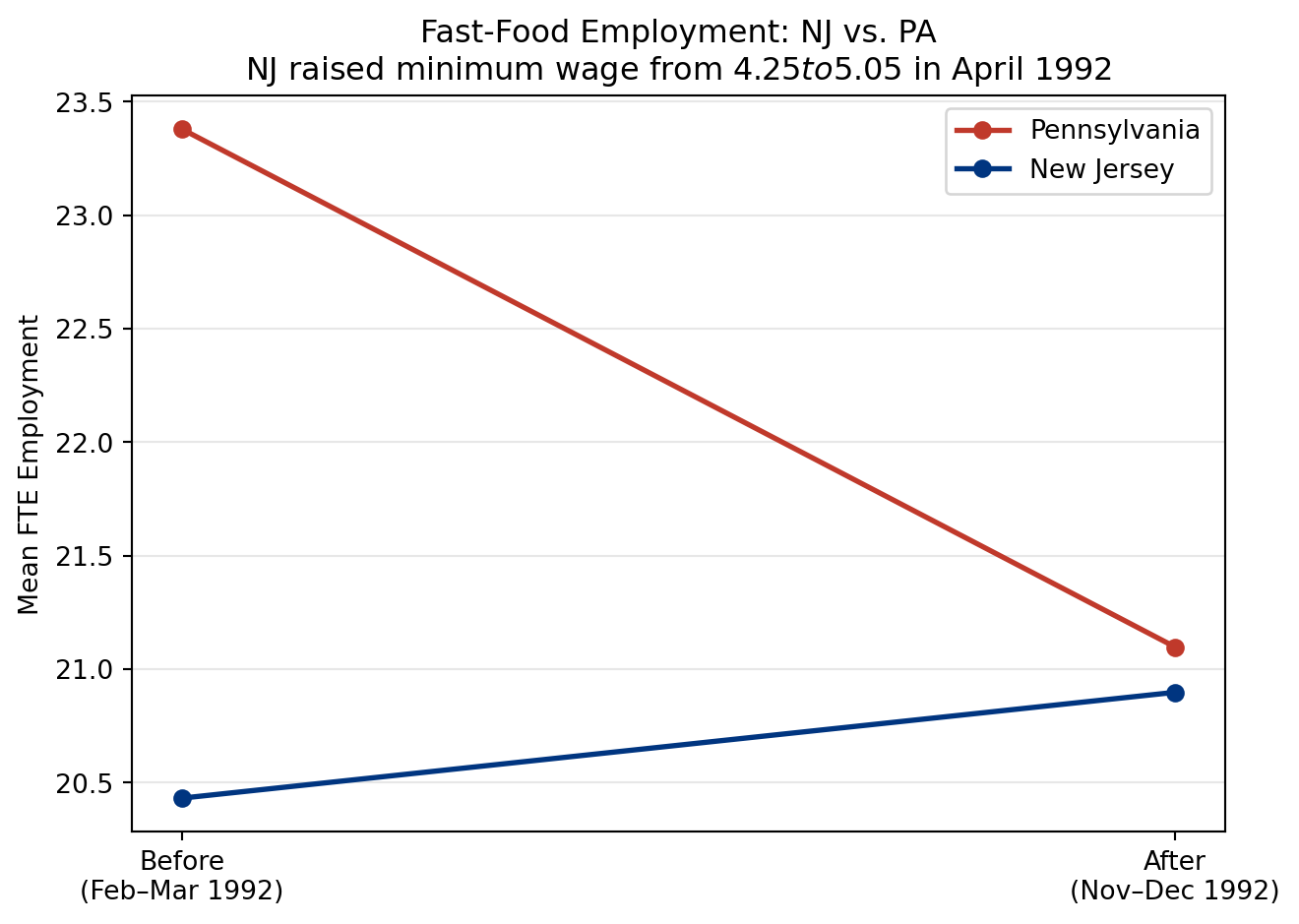
df["nj"] = df["STATE"]  # 1 = New Jersey, 0 = Pennsylvania

# FTE employment = full-time + 0.5 * part-time + managers
df["fte_before"] = df["EMPFT"] + 0.5 * df["EMPPT"] + df["NMGRS"]
df["fte_after"]  = df["EMPFT2"] + 0.5 * df["EMPPT2"] + df["NMGRS2"]
df["change_fte"] = df["fte_after"] - df["fte_before"]

# Meal price = soda + fries + entree
df["meal_price"]  = df["PSODA"] + df["PFRY"] + df["PENTREE"]
df["pct_ft"]      = df["EMPFT"] / df["fte_before"] * 100

# Drop stores missing employment data in either wave
df = df.dropna(subset=["fte_before", "fte_after"])

print(f"Stores in sample: {len(df)}")
print(f"  Pennsylvania: {(df['nj'] == 0).sum()}")
print(f"  New Jersey:   {(df['nj'] == 1).sum()}")
Stores in sample: 384
  Pennsylvania: 75
  New Jersey:   309

Main Analysis

Table 2 (Selected Rows): Pre-Period Store Characteristics

Table 2 in the paper shows characteristics of stores before the April 1992 minimum wage change. NJ stores were already paying slightly higher wages on average, and had lower FTE employment than PA stores.

# Compute means by state for the pre-period
table2 = df.groupby("nj").agg(
    stores      = ("SHEET",      "count"),
    wage        = ("WAGE_ST",    "mean"),
    fte         = ("fte_before", "mean"),
    pct_ft      = ("pct_ft",     "mean"),
    meal_price  = ("meal_price", "mean"),
    hours_open  = ("HRSOPEN",    "mean")
).reset_index()

table2.index = ["Pennsylvania", "New Jersey"]
table2 = table2.drop(columns="nj")
table2.columns = ["Stores (N)", "Starting Wage ($)", "FTE Employment",
                  "% Full-Time", "Meal Price ($)", "Hours Open"]

print(table2.round(2).to_string())
              Stores (N)  Starting Wage ($)  FTE Employment  % Full-Time  Meal Price ($)  Hours Open
Pennsylvania          75               4.63           23.38        35.26            3.06       14.51
New Jersey           309               4.61           20.43        32.63            3.36       14.40

Table 3 (Panel A, Columns 1–3): Difference-in-Differences

This is the central result. The table shows average FTE employment before and after the wage increase for each state, the within-state changes, and the DiD estimate in the bottom-right corner.

pa = df[df["nj"] == 0]
nj = df[df["nj"] == 1]

# Means
pa_before = pa["fte_before"].mean()
nj_before = nj["fte_before"].mean()
pa_after  = pa["fte_after"].mean()
nj_after  = nj["fte_after"].mean()
pa_change = pa["change_fte"].mean()
nj_change = nj["change_fte"].mean()

# Standard errors for the differences
def diff_se(a, b):
    se_a = a.std() / np.sqrt(len(a))
    se_b = b.std() / np.sqrt(len(b))
    return np.sqrt(se_a**2 + se_b**2)

se_before = diff_se(nj["fte_before"], pa["fte_before"])
se_after  = diff_se(nj["fte_after"],  pa["fte_after"])
se_change = diff_se(nj["change_fte"], pa["change_fte"])

table3 = pd.DataFrame({
    "Pennsylvania": [pa_before, pa_after, pa_change],
    "New Jersey":   [nj_before, nj_after, nj_change],
    "NJ − PA":      [nj_before - pa_before, nj_after - pa_after, nj_change - pa_change],
    "SE (NJ−PA)":   [se_before, se_after, se_change]
}, index=["FTE before", "FTE after", "Change in FTE"])

print(table3.round(2).to_string())
               Pennsylvania  New Jersey  NJ − PA  SE (NJ−PA)
FTE before            23.38       20.43    -2.95        1.48
FTE after             21.10       20.90    -0.20        1.10
Change in FTE         -2.28        0.47     2.75        1.34

The bottom-right cell — the DiD estimate — shows that NJ stores saw employment rise by roughly 2.76 FTE employees relative to PA stores after the minimum wage increase.

Something Additional

Table 4, Column (i): Formalizing the DiD as a Regression

The DiD estimate can be expressed as a simple OLS regression:

\[\Delta \text{FTE}_i = \alpha + \beta \cdot \text{NJ}_i + \varepsilon_i\]

The intercept is the average employment change in PA (the control baseline), and \(\beta\) is the extra change in NJ — the same number as the DiD estimate above.

model = smf.ols("change_fte ~ nj", data=df).fit()

# Pull out just the key results
results = pd.DataFrame({
    "Estimate":   model.params,
    "Std. Error": model.bse,
    "t-stat":     model.tvalues,
    "p-value":    model.pvalues
})
results.index = ["Intercept (PA avg. change)", "NJ indicator (β)"]

print(results.round(3).to_string())
                            Estimate  Std. Error  t-stat  p-value
Intercept (PA avg. change)    -2.283       1.036  -2.205    0.028
NJ indicator (β)               2.750       1.154   2.382    0.018

The \(\beta\) coefficient matches the DiD number from Table 3 exactly. The intercept of roughly −2.16 is the average employment decline in Pennsylvania over the same period — the trend that NJ avoided.

Visualizing the DiD

fig, ax = plt.subplots(figsize=(7, 5))

periods = ["Before\n(Feb–Mar 1992)", "After\n(Nov–Dec 1992)"]

ax.plot(periods, [pa_before, pa_after], marker="o", linewidth=2,
        color="#c0392b", label="Pennsylvania")
ax.plot(periods, [nj_before, nj_after], marker="o", linewidth=2,
        color="#003580", label="New Jersey")

ax.set_ylabel("Mean FTE Employment")
ax.set_title("Fast-Food Employment: NJ vs. PA\nNJ raised minimum wage from $4.25 to $5.05 in April 1992")
ax.legend()
ax.grid(axis="y", alpha=0.3)

plt.tight_layout()
plt.show()

Why Difference-in-Differences Enables a Causal Claim

The fundamental challenge is that NJ and PA differ in many unobservable ways — local demand, demographics, chain composition. A naive before/after comparison for NJ alone would confound the wage policy with any macro shocks that happened to hit between the two survey waves.

DiD solves this by subtracting the PA trend from NJ’s change. Any shock that affected both states equally — a national slowdown, seasonal patterns, industry-wide pressures — cancels out of the difference. The residual is attributed to the policy.

The design is especially credible here because:

  1. Geographic proximity: NJ and PA border each other, making them similar on many dimensions that are hard to measure.
  2. Exogenous timing: the wage increase was legislated well in advance; restaurants didn’t choose when it took effect.
  3. Pre-period comparability: as Table 2 shows, the two states had similar store characteristics before the change, lending credibility to the parallel-trends assumption that underlies the whole design.